Time at the Bar Chart

This is part three in a blog mini-series about the power of Streaming Platforms with Kafka, KSQL and Confluent.

Part 1 was an introduction to the problem of converting events to models in real time Part 2 showed how we can do that conversion using Kafka, Streams and KSQL Remember that code can be downloaded from my github.

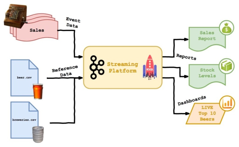
This post is all about aggregations. Looking at how we can get aggregated data out of the streaming platform both real-time and ad-hoc style. Here’s a reminder of the Beer Festival simulation I’ve been using:

Two full days of work went into the job of extracting results from Kafka and displaying them on a chart! I might write another article about how difficult it was, but for now we’re just going to talk about aggregations in KSQL and forget the last 48 hours ever happened… OK?

Sales Report

In order to understand profitability and bar utilisation, as organiser of the beer festival, I want to see real time information on sales, aggregated by bar number.

ksql> create stream live_sales \
with (kafka_topic='live_sales', value_format='avro', partitions=4) \
as select * from sales_stream;

ksql> create table takings_by_bar \
with (kafka_topic='takings_by_bar', value_format='avro') \
as select bar, sum(price) as sales from live_sales group by bar;

Writing the KSQL to do an aggregation is pretty simple. Here I group by bar and return sum(price), just like in regular SQL. I also created a new stream called “live_sales” with 4 partitions, so we can do joins later. These query results gets rolled up into a table, from which we can select:

ksql> select * from takings_by_bar;
1543263893133 | 1 | 1 | 16110
1543263895143 | 2 | 2 | 12162
1543263896149 | 1 | 1 | 16111
1543263897153 | 3 | 3 | 8361
1543263899164 | 3 | 3 | 8362
1543263898158 | 2 | 2 | 12163
1543263900168 | 1 | 1 | 16113
1543263901175 | 4 | 4 | 4147

The results of the select, however, are not what we might immediately expect. Rather than a row for every bar (four rows total) we’re getting what look like duplicates. This is because the table is based on a stream of sales messages: the value of count(*) changes every time a new sale is recorded, and KSQL returns the updated value each time this happens.

If I stop the flow of sales records, by killing the producer, and tell KSQL to read the table from the start, I get more ’normal’ looking results:

ksql> SET 'auto.offset.reset' = 'earliest';

ksql> select * from takings_by_bar;
1543264451505 | 2 | 2 | 12354
1543264452513 | 4 | 4 | 4218
1543264444458 | 3 | 3 | 8496
1543264450501 | 1 | 1 | 16409

Obviously, the beer festival can’t pause every time the organisers want to draw a bar chart, so I added a little dictionary-based cache between Kafka and the front end. You can find the code for my simple caching web service on Github as always.

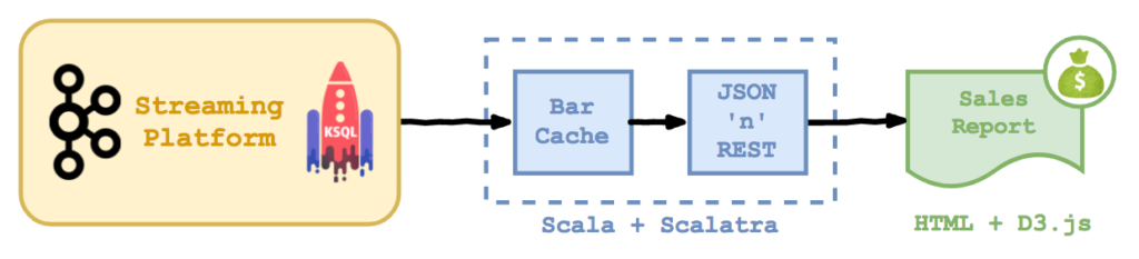
The middle-tier is a basic self-contained REST service based on Scalatra, the world’s leading web micro-framework for Scala. The front-end is a D3.js chart (code here), which pulls data from the middle tier in JSON format.  I’m not recommending this as a production architecture, but it’s a nice demo!

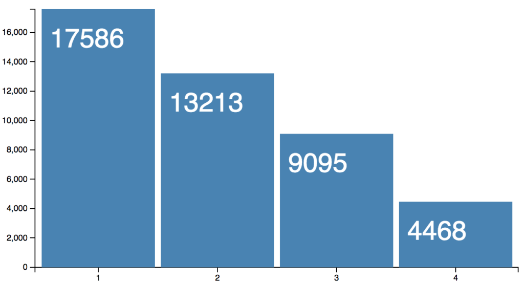
The beer festival has been running for a few days now, bar 1 is clearly nearer the door, while, tucked away behind the pork scratching stand, bar 4 is only selling pilsners.

Windowed Aggregations

In order to understand the rate of beer sales, right now, as a beer festival organiser, I want to see the sales per bar, for the last minute only.

The bar chart in the previous part showed the sales for all time. This isn’t much use if we want to see what’s happening right now. So, let’s create another aggregated table to show the total beer sales, by bar for the last minute:

ksql> create table takings_by_bar_last_min \
with (kafka_topic='takings_by_bar_last_min', value_format='avro', partitions=1) \
as select bar, sum(price) as sales \
from live_sales window tumbling (size 1 minute) \
group by bar;

The interesting bit in the query above is “window tumbling” which creates a one minute aggregation window. When the minute elapses, the window closes and a new one opens, with the counts starting at zero again. Here’s a screenshot… everything else is the same, really.

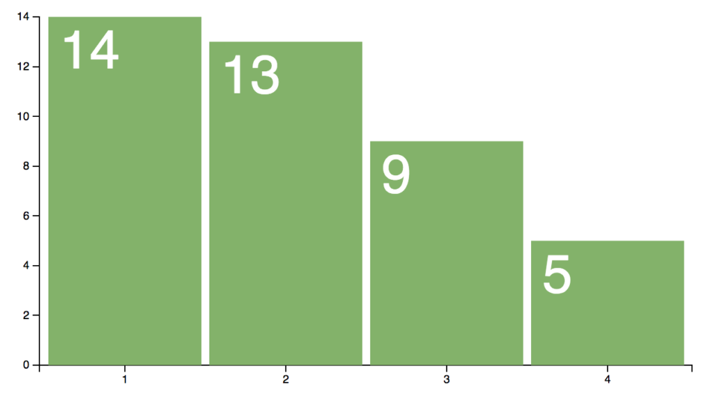
Note that you can also do ‘hopping’ and ‘session’ windows which slide the window in smaller increments and lock windows to sessions, respectively. Tumbling works fine for the beer festival though.

Top 10 Beers

In order to see which beers are a hit with the punters, as a broadcaster providing commentary on International Real Ale TV, I want to see a live league table of the top 10 best selling beers.

Let’s jump straight in with a join, to get beer names and sales into a stream together…

ksql> create stream live_beer_sales \
with (kafka_topic='live_beer_sales', value_format='avro') \
as select bar, price, name, abv from live_sales LS \
join beer_table BT on (LS.beer_id = BT.id);

ksql> select * from live_beer_sales limit 4;
1543303642980 | 1465 | 2 | 1 | Granny Smith Hard Apple Cider | 0.069
1543303643997 | 1543 | 1 | 1 | Proxima IPA | 0.063
1543303645003 | 1098 | 1 | 2 | Hala Kahiki Pineapple Beer | 0.048
1543303646017 | 1957 | 1 | 1 | 805 Blonde Ale | 0.047

Getting the total numbers of each beer sold is easy - as you can see from the snippet below. We just group the joined sales data by name and sum the price to get the total sales. Note the funky key column for the table, which is the name and ABV concatenated (since I needed both in the results and they are covariant I just grouped by both).

ksql> create table beer_league_table \
with (kafka_topic='beer_league_table', value_format='avro') \
as select name, abv, sum(price) as sales \
from live_beer_sales group by name, abv;

ksql> select * from beer_league_table limit 4;
1543303572099 | Nordic Blonde|+|0.057 | Nordic Blonde | 0.057 | 1
1543303618561 | Black Beer`d|+|0.068 | Black Beer`d | 0.068 | 1
1543303630874 | Mustang Sixty-Six|+|0.05 | Mustang Sixty-Six | 0.05 | 1
1543303651048 | Dubbelicious|+|0.065 | Dubbelicious | 0.065 | 1

Here comes the tricky part though. KSQL does have a function called ‘TOPK’ which will return the top k values for a given column. However, this will only return the counts, not the associated rows. Since it doesn’t help us much to show only counts, I’m just going to do the sort on the client side!

You can find the code for the chart here.

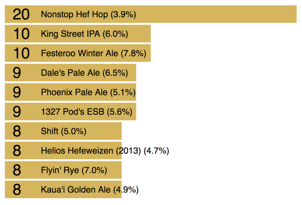
It’s a shame you can’t see the chart moving, because it animates beautifully!

Time at the Bar Chart

So that was a very swift tour of some of Kafka and KSQL’s aggregation functionality, combined with joins to reference data and schema transformation too. All in all I’m very happy with the results and we’re now pretty much all the way through our use-case.

One thing I was reminded of, while writing this blog, is that KSQL may make Kafka look like a bunch of tables, but it is most definitely a streaming platform under the hood. Though we can use KSQL to turn our events into models, squashing updates into single records and joining streams together, we’re still going to need to write the output to a real database at some point if we want to do traditional reporting.

That said, I was able to create two or three real-time reports in just a few hours, with minimal code (ignoring the time I spent working out how to do it!). The charts look great and the web services I wrote are basic, but could be productionised pretty easily. All in all, it’s been great - I hope you enjoyed it too!