Face Clustering with Python

This journey began with a conversation - maybe a debate - with this guy who works for a makeup company.  We were talking about how makeup artists will match a finite set of “looks” to people’s faces, based on a simple set of attributes.  I can’t remember the precise attributes, but along the lines of “big forehead”, “rounded jaw”, “small nose” etc. My gut feel, at the time, was “this sounds easy!” and thus I set forth on a voyage of discovery…

That evening I got home, fired up PyCharm and thought about the things I’d need to prove my point:

• A database of faces, to use to test my code
• A python library for detecting the features of people's faces
• A simple algorithm for clustering the faces, based on their features
• Some way to display the results, to validate the approach

Just for the record, I never saw the guy I’d originally chatted to again. I continued on my journey, motivated only by a quest for self fulfilment!

A Database of Faces

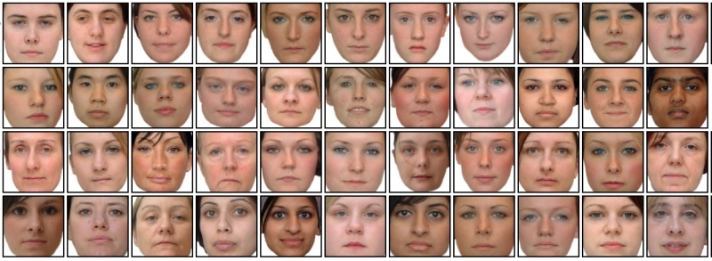
Finding a database of faces turned out to be pretty simple.  I wanted to use a freely-available collection of varied faces, where each person’s face was posed in a pretty standard way: a neutral expression, looking straight towards the camera; consistent lighting… you get the idea.

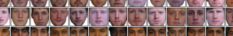
In the end, I discovered The Glasgow Unfamiliar Face Dataset, which contains a reasonable number of photos of faces, for women and men.  I used the women’s faces for the majority of work.  Statistically speaking, women are more likely to wear makeup, so if this dude’s theory is true, he’s probably talking about women’s faces, and that’s how this started.

Face Detection Library

So, having filled my laptop with unfamiliar faces, the next step was to see if I could detect some features in those faces.  Get the coordinates of the nose, the eyes, the jawline and so on.  Of course there’s a library to do this in Python, in fact there are several.  I started with the DLib and opencv libraries, following this epic tutorial.  I won’t duplicate the code here, as I didn’t add much.  Suffice it to say that within an hour or so (mostly wrestling installers on my macbook) I was able to detect features in faces like this:

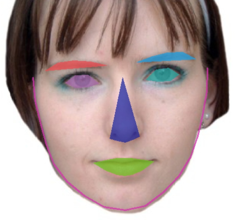
So this cool set of library calls allows me to turn a photo of a face into a list of coordinates for points within facial features.  Basically projecting down a very complex blob of pixel data into a smaller set of coordinate data.  Supercool!  But not good enough for clustering yet.  The first issue is that the coordinate data is in pixel coordinate space, so it’s heavily influenced by the location of the face in the photo.  If we were to cluster using this data we’d group people by their location in a photo, not by any property of their face.

>>> print(features)
[[ 83 348], [ 87 392], [ 97 434], [108 474], [122 511], [147 544], [180 571] ... [301 508], [268 509], [255 512], [241 510]]

At this point, as I often do, I decided to try the simplest, easiest technique I could think of to normalise my feature data using brute force.  I started off this post talking about features like “nose size” and “jaw width” as those are features of a human face we can all understand… and with all this coordinate data they are easy to calculate too.  Here’s an example:

<em># Get the nose features
</em>(i, j) = face_utils.FACIAL_LANDMARKS_IDXS[**"nose"**]
nose_points = shape[i:j]
nose_top = nose_points[self.NOSE_TOP_IDX]
nose_left = nose_points[self.NOSE_LEFT_IDX]
nose_right = nose_points[self.NOSE_RIGHT_IDX]
nose_bottom = nose_points[self.NOSE_BOTTOM_IDX]
nose_width = distance.euclidean(nose_left, nose_right)
nose_height = distance.euclidean(nose_top, nose_bottom)
nose_ratio = nose_height / nose_width
nose_size = nose_height / jaw_width

This is just a snippet of the feature detection code I sweated out that evening!  First I extracted the nose points, then I got the top-, left-, bottom- and right-most points, then I calculated the pixel height and width and finally and critically, normalised these by dividing through by the jaw width.

Expressing all the feature sizes in proportion to some arbitrary measurement of the face (in this case I chose the jaw width) moves us from pixel-space to… erm… face-space.  Now we can compare nose sizes with some level of fairness.  I expressed eight easy measurements this way to create a feature vector for every face in my database.

face_data = {
    **"filename"**: **"faces/" **+ filename.split(**'/'**)[-1],
    **"features"**: [
        jaw_ratio,
        eye_distance,
        nose_ratio,
        nose_size,
        eye_size,
        eye_size_differential,
        eyebrow_width,
        eyebrow_lift
    ]
}

A vector representation of a face, in the world of image recognition, is known as an ‘Embedding’.  What I have shown here is basically the simplest, crudest and most embarassingest technique for generating an embedding from a face image.  Go me!

Clustering

So now we have a crude set of embeddings for our sample image data, let’s employ a crude clustering algorithm and see what happens.  By this stage my journey had entered it’s second day.  It’s rare for me to code on a weekend these days, but this was just too interesting!

K-Means

Everyone knows it, the easiest way to cluster vectors of data is to use K-Means.  It’s even easier in Python, where the libraries do all the hard work for you.

Imagine you have some objects, each of which is represented by a vector of numeric values.  It could be anything: rows in a spreadsheet, house prices, salaries, ages or (bet you saw this coming…) crude measurements of a face.  Each of these vectors describes a point in n-dimensional space.  Easy to imagine if you have one, two or three values - so keep a 3D space in your head and don’t give yourself an 8-dimensional headache.  Now imagine you randomly choose a set number (k) of “centres” in the same n-dimensional space.  Now you can associate points with their nearest cluster, then move the cluster centres closer to their associated points, then iterate.  Points attract centres, centres group points, eventually the cluster centres creep into the right places and, when they stop moving, define the discreet clusters in our data.  Boom!

generate k random cluster centres

assign every point to the **nearest** cluster centre

do { 
    move every cluster centre closer to it's associated points

    assign every point to the nearest cluster centre again

} while (something changed)

I used the Scikit Learn implementation of K-means to do my clustering.  Here’s a snippet:

**import **numpy **as **np
**from **sklearn.cluster **import **KMeans

<em># Get the face data
</em>data = [np.array(face[**"features"**]) **for **face **in **faces]

<em># Build the model using the face data
</em>kmeans = KMeans(n_clusters=cluster_count)
kmeans = kmeans.fit(data)

<em># Get cluster numbers for each face
</em>labels = kmeans.predict(data)
**for **(label, face) **in **zip(labels, faces):
    face[**"group"**] = int(label)

Choosing K

The problem with K-Means clustering is that it’s hard to know what value of k to use - how many clusters naturally exist in your data?  One way to find out is to look at the cost function.  For any given value of k, you can look at the distance between elements and cluster centres.  As the value of k increases this distance will obviously decrease, until k is equal to the number of rows in your dataset, when the cost is 0.

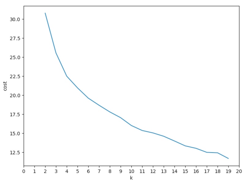
What we’re looking for in the above chart is an “elbow” - a point where adding more cluster centres (increasing k) adds less benefit.  I think there’s an elbow around k=4 - but it’s vague, which is not promising.

First Set of Results

So here is the first set of results - shown in a very simple D3js table.  I set k to 4, based on the analysis above.

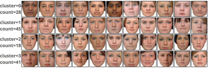
I have stared at the results for ages - sometimes I can see similarities between the faces and sometimes I can’t.  Smaller noses on the top row, longer noses on row three? Eyes further apart on the bottom row?  You can draw your own conclusions about whether this worked or not!

Given that the success or failure of this exercise is so subjective, and I haven’t got time to devise a similarity test to validate the results with human input, I decided I needed a dataset I knew better.

So, if the algorithm can cluster people by properties of their faces, and I present it with a dataset of known faces… maybe the faces of my family… I know there are four of us… so if I set k=4 and present my holiday photos the clustering should group each of the four of us into a distinct cluster…

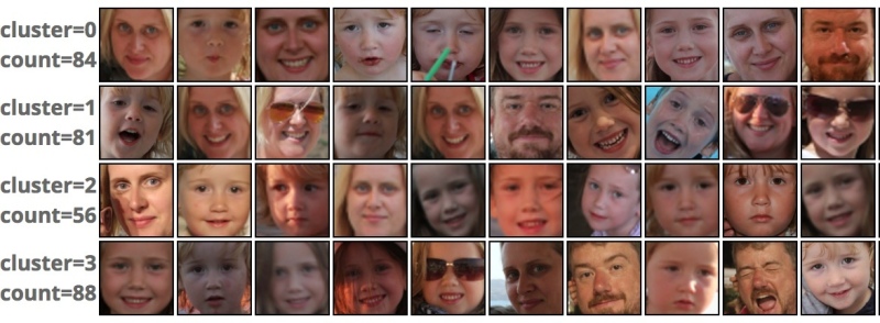
Oh dear!  That doesn’t look so good does it!  It’s pretty much a random shuffle of the four of us.  There are all sorts of possible reasons for this - the most likely being the noisy nature of the input data.  Loads of sunglasses, daft expressions, funny angles, weird lighting and so on.  Given that I’m directly measuring facial features I’m bound to be prone to issues when people pull a funny face… or just smile!

So What?

That’s it for Part 1 I think.  So what did I learn?  Well, I reaffirmed my belief that there is a Python library for literally everything and that, in a few hours, it’s very easy to do some preliminary hacking around some hypothesis you may have - and learn something in the process.

I learned that detecting features and generating an embedding from a bitmap image is* exactly as easy as I thought*, and that the real challenges with image recognition are not in the low level mechanics (measuring a nose for example) but in the subtle details of a smile or a frown.

With the neutral expressions of the Unfamiliar Faces, I do feel I had some success - however hard this might be to prove.  With family member recognition it was a total fail.

In part 2 I’ll explain how I took this further, using an off-the-shelf Neural Network to generate a better embedding which gave amazing results, even when sticking with basic k-means clustering.